SHAP (SHapley Additive exPlanations) is a unified approach to explain the output of any machine learning model.

It combines game theory with machine learning models.

It has optimized functions for interpreting tree-based models and a model agnostic explainer function for interpreting any black-box model for which the predictions are known.

In summary, Shapley’s values calculate the importance of a feature by comparing what a model predicts with and without this feature. However, since the order in which a model sees the features can affect its predictions, this is done in all possible ways, so that the features are compared fairly. This approach is inspired by game theory.

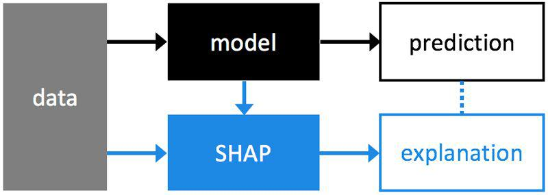
SHAP is used to explain an existing model. Take a binary classification case built with sklearn for example. We train, tune and test our model. Then we can use our data and the model to create an additional SHAP model that explains our classification model.

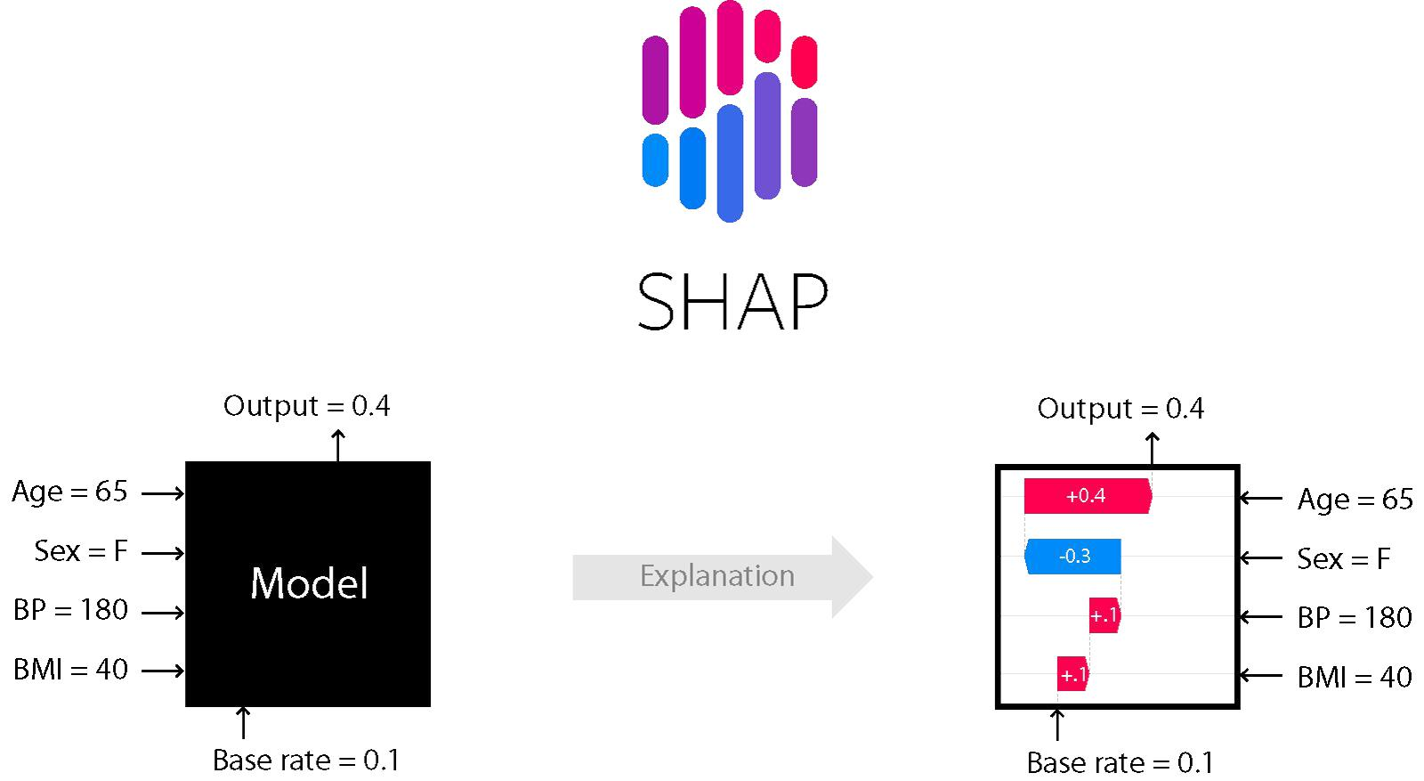
Look at how every feature is assigned a weight/importance score by SHAP:

SHAP builds model explanations by asking the same question for every prediction and feature:

“How does prediction i change when feature j is removed from the model?”

The so-called SHAP values are the answers.

They quantify the magnitude and direction (positive or negative) of a feature’s effect on a prediction.

1. Missingness: If the simplified inputs represent feature presence, then missingness requires features missing in the original input to have no impact.
2. Consistency: Consistency states that if a model changes so that some simplified input’s contribution increases or stays the same regardless of the other inputs, that input’s attribution should not decrease.
3. Efficiency: As the foundation of SHAP values is based on computational game theory, this is the only method that can fairly distribute the gain of the feature.
4. Global comparison: SHAP values provide a way to compare the feature importance at a global level. You can also change the dataset from global to a subset dataset of interest.

1. Computation time: Number of possible combinations of the features exponentially increases as more number of features are added. This in turn increases the turn around time of calculating SHAP values, and approximation is the only solution.
2. Order of feature selection in all possible combinations: Typically while solving real world problems, the target is non-linearly related with the independent features, and there is some correlation amongst the independent features too. In such cases the order in which the features are selected in the combination matters, and can impact the SHAP values.
3. Simulation of scenarios: SHAP doesn’t return a model, like LIME. So if you want to simulate scenarios to see how much the output is impacted by increase in a particular feature, then it’s not possible with SHAP.
4. Correlation amongst independent features: Again in most real world problems the independent features will be correlated. In such situations, when we sample from feature’s marginal distribution, there can be instances generated which might not be possible in real world.

It is important to understand all the bricks that make up a SHAP explanation.

• global explanations: explanations of how the model works from a general point of view.
• local explanations: explanations of the model for a sample (a data point).
• explainer (shap.explainer_type(params)): type of explainability algorithm to be chosen according to the model used.
  The parameters are different for each type of model. Usually, the model and training data must be provided, at a minimum.
• base value (explainer.expected_value): E(y^) is “the value that would be predicted if we didn’t know any features of the current output”. It is the mean of y for the training data set or the background set. We can call it “reference value”, it’s a scalar (n).
• SHAPley values (explainer.shap_values(x)): the average contribution of each feature to each prediction for each sample based on all possible features. It is an n×m matrix that represents the contribution of each feature to each sample.
• output value (for a sample): the value predicted by the algorithm (the probability, logit or raw output values of the model).
• display features (n×m): a matrix of original values — before transformation/encoding/engineering of features etc. — that can be provided to some graphs to improve interpretation. Often overlooked and essential for interpretation.

There’s NO need to worry if you don’t understand all these terms completely. If you want to understand the meaning of something during the implementation, you can simply come back and refer to this.

The SHAP library offers different visualizations.

• To date, force plots have been the default method for visualizing individual model predictions.
• SHAP decision plots show how complex models arrive at their predictions (i.e., how models make decisions).
• The summary plot shows the most important features and the magnitude of their impact on the model. It can take several graphical forms and for the models explained by TreeExplainer we can also observe the interaction values using the “compact dot” with shap_interaction_values in input.
• The dependency plot allows us to analyze two features at a time by suggesting a possibility to observe the interactions. The scatter plot represents a dependency between a feature(x) and the shapley values (y), colored by a second feature(hue).

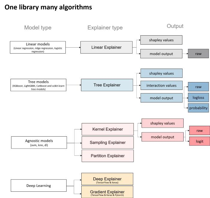
Explainers are the models used to calculate shapley values. The diagram below shows different types of Explainers.

The choice of Explainers depends mainly on the selected learning model:

• For linear models, the “Linear Explainer” is used.
• For decision trees and “set” type models — “Tree Explainer” can be used. In addition the “Tree Explainer” allows to display the interaction values. It also allows to transform the model output into probabilities or log-loss, which is useful for a better understanding of the model or to compare several models.
• “Kernel Explainer” can be used on all models — either tree or non-tree based. However, it is slower than the above mentioned explainers. It creates a model that substitutes the closest to our model. Kernel Explainer can also be used to explain neural networks.
• For deep learning models, there are the Deep Explainer and the Gradient Explainer.
• All the explainers are explained in detail here: https://shap.readthedocs.io/en/latest/examples.html#general

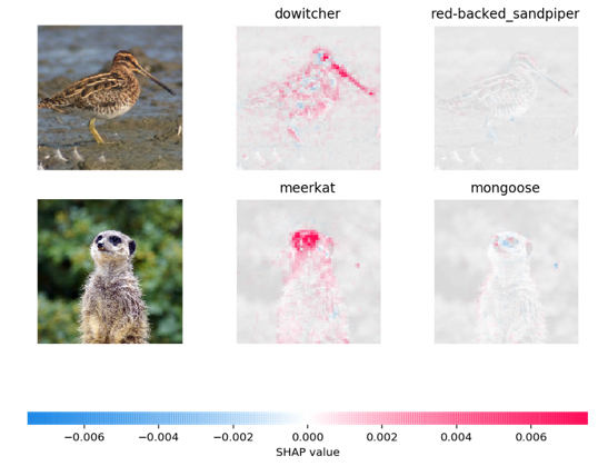
The SHAP package is also useful in other machine learning tasks as well. For example, image recognition tasks or text-based tasks. In the figure below, you can see which pixels contributed to which model output: